Contour Plot of pollutant concentration field — contourPlot2 • simulariatools

The function contourPlot2 generates a contour plot of a scalar quantity, such as the ground concentration of an airborne pollutant or odour, defined on a regular grid.

Usage

contourPlot2(
  data,
  x = "x",
  y = "y",
  z = "z",
  domain = NULL,
  xlim = NULL,
  ylim = NULL,
  nticks = 5,
  background = NULL,
  basemap = NULL,
  underlayer = NULL,
  overlayer = NULL,
  legend = NULL,
  levels = NULL,
  size = 0,
  fill = TRUE,
  tile = FALSE,
  transparency = 0.75,
  colors = NULL,
  mask = NULL,
  inverse_mask = FALSE,
  bare = FALSE,
  theme_void = FALSE
)

Arguments

data: A dataframe in long format with three columns for Easting, Northing and values to be plotted.
x: character. Name of the column containing Easting (longitude) coordinates (default "x").
y: character. Name of the column containing Northing (latitude) coordinates (default "y").
z: character. Name of the column containing concentration values (default "z").
domain: optional list of six numeric values defining the boundaries of the domain to be plotted and the number of ticks on X & Y axis (minimum X, maximum X, minimum Y, maximum Y, number of ticks on X axis, number of ticks on Y axis). Example: c(340000, 346000, 4989500, 4995500, 5, 5). If missing, the full domain of the input data is considered, with 5 ticks (deprecated, see xlim, ylim, nticks).
xlim: optional list of two numeric values defining the abscissa axis boundaries of the plot (minimum x, maximum x).
ylim: optional list of two numeric values defining the ordinate axis boundaries of the plot (minimum y, maximum y).
nticks: optional list of one or two numeric integers defining the number of ticks on X & Y axes. If a single number is given, the same number of ticks is plotted on both axes (default = 5 ticks).
background: filename. Optional path to a raster file to be plotted as the basemap (deprecated, see basemap)
basemap: filename. Optional path to a raster file to be plotted as the basemap (see Details).
underlayer: optional list of layers to be plotted between basemap and contour plot. See Details.
overlayer: optional list of layers to be plotted on top of the contour plot. See Details.
legend: character. Optional title of the legend.
levels: numeric vector of levels for contour plot. If not set, automatic pretty levels are computed. If -Inf and Inf are used as the lowest and highest limits of the array, the lowest and highest bands are unbounded and the legend shows < and >= symbols.
size: numeric. Width of the contour line.
fill: logical. If TRUE, the contour plot is filled with colour (default = TRUE).
tile: logical. If TRUE, rectangular tiles are plotted (default = FALSE).
transparency: transparency level of the contour plot between 0.0 (fully transparent) and 1.0 (fully opaque). Default = 0.75.
colors: colour palette for contour plot, as an array of colours.
mask: character. Path to shp file used as a mask. It must be a closed polygon.
inverse_mask: logical. If TRUE, areas on mask are masked. Default is to mask areas outside the polygon defined in the shp file.
bare: boolean (default FALSE). Deprecated in favour of theme_void.
theme_void: boolean (default FALSE). If TRUE, only the bare plot is shown: axis, legend, titles and any other graphical element of the plot are removed.

Value

A ggplot2 object.

Details

This is a convenience function to plot contour levels of a scalar quantity such as pollutants computed by a dispersion model, with ggplot2 version >= 3.3.0.

Data are required to be on a regular grid, typically (but not necessarily) in UTM coordinates. Each value is associated to the cell centre. The input dataframe has to be in long format, i.e. one line per value to be plotted. The names of the columns corresponding to x, y and z can be specified in the input parameters.

The basemap can be a geo-referenced TIFF file. In that case, the plot bounding box is automatically derived from the picture extent. The axis limits can be explicitly overridden by xlim and ylim arguments.

If tile = TRUE data are shown as they are, without any graphical interpolation required for contour plots. This is helpful when you want to visualise the raw data. Since version 2.4.0, when tile = TRUE the intervals include the lowest bound and exclude the highest bound: [min, max). Note: In previous versions it was the opposite.

underlayer and overlayer layers are ggplot2 objects to be shown at different levels of the vertical stack of the plot. These are useful to show topographical information related to the plot, such as sources or receptors locations.

When a shp file is given to the mask argument, the plot is drawn only inside the polygon. In order to avoid boundary artifacts due to reduced resolution, original data are resampled to higher resolution (currently set to 10 times the original one). If inverse_mask is set to TRUE, the plot is drawn outside the polygon. The mask feature is based on the terra::mask() function. The CRS of the shp file is applied to the data in the data.frame. Please keep in mind this feature is still experimental.

Examples

# Load example data in long format
data(volcano)
volcano <- as.data.frame(volcano)
volcano3d <- reshape(volcano, direction = "long",
  varying = list(1:61),
  idvar = "x", timevar = "y", v.names = "z")
# Contour plot with default options
v <- contourPlot2(volcano3d)
v


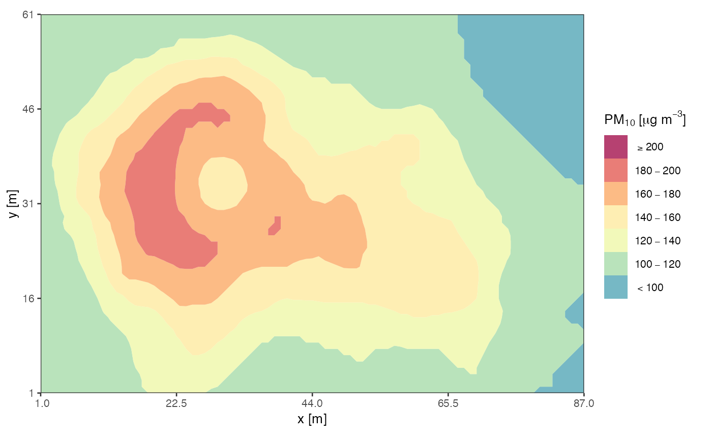
# Set levels, and properly format the legend title:
contourPlot2(
    volcano3d,
    levels = c(-Inf, seq(100, 200, 20), Inf),
    legend = expression("PM"[10] ~ "[" * mu * "g m"^-3 * "]")
)


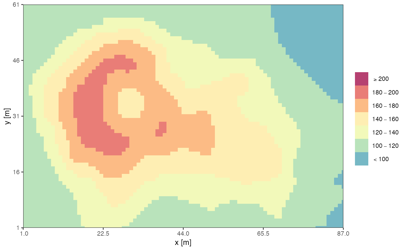
# Sometimes, instead of a contour plot it is better to plot the original
# raster data, without any interpolation:
contourPlot2(
    volcano3d,
    levels = c(-Inf, seq(100, 200, 20), Inf),
    tile = TRUE
)


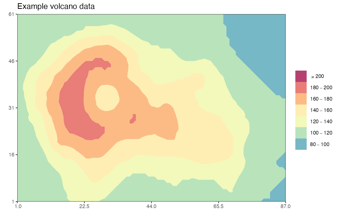
# Since contourPlot2 returns a `ggplot2` object, you can add instructions as:
library(ggplot2)
v +
    ggtitle("Example volcano data") +
    labs(x = NULL, y = NULL)